Approximations of Errors in Measurement

1. Approximations

If a quantity x (eg, side of a square) is obtained by measurement and a quantity y (eg, area of the square) is calculated
as a function of x, say y = f(x), then any error involved in the measurement of x produces an error in the calculated
value of y as well.

Suppose the distance x_m between 2 points is measured be 1000m with an error of 1m. this means that the measured distance x_m is 1000m: x_m= 1000 and the actual distance x_a is somewhere between 1000m-1m= 999m and 1000+1m=1001m; it`s somewhere the interval [999,1001]. We say that the distance is measured to be 1000m and 1000m+1m. The error of 1m is how much x_a can differ from x_m :| x_a- x_m |=1. Now x_m and x_a are 2 particular values of variable say x. more precisely x_m is a value of x and x_a is a value which x can change from x_m to. So the error of 1m can be considered as a change in x

The error can be considered as a change in x_, and thus is denoted by Dx, consequently the error in x is Dx=dx. The corresponding error in y is Dy= f(x+dx)-f(x), and the corresponding differential of f ay x is dy=f’(x)dx, intuitively we can approximate Dy by dy. Now let`s show we can do such an approximation.

But we have that f(x+dx)@ f(x) + f’(x)dxà Dy= f(x+dx)- f(x) @ (f(x) + f’(x)dx)-f(x)

Indeed we can approximate Dy by dy, intuitively approximating the height of the graph of f by that of the tangent amounts to approximating the length Dy by the length dy, as clearly seen in the fig. 1.1

In summary: Dx= dx, Dy@ dy= f’(x)dx

That is, the error in x is dx and the corresponding approximate error in y is dy = f '(x) dx.

Fig. 1.1

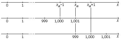
As seen above we say that the distance between 2 points is measured to be 1000m ± 1m its measurent is 1000m with an error of 1m. the measured distance is x=1000, the error is dx =, and the actual distance x_a is somewhere in the interval [1000-1,1000+1]= [999,1001]. If instead interpret differently by treating that x_a is such that x=1000 is somewhere in the interval [x_a-1, x_a+1] so we get this 999≤ x_a ≤1001, i.e. x_a is somewhere in the interval [999,1001], the same situation as in the 1^st interpretation. Fig.1.2

Fig. 1.2 – 1st and 2nd axes: if 1,000 = xa – 1 then xa = 1,001, – 1st and 3rd axes: if 1,000 = xa + 1 then xa = 999, therefore xa is somewhere in [999, 1,001].

2. Types of Errors

A measurement of distance d₁ yields d₁ = 100 m with an error of 1 m. A measurement of distance d₂ yields d₂ = 1,000 m
with an error of 1 m. Both measurements have the same absolute error of 1 m. However, intuitively we feel that
measurement of d₂ has a smaller error because it's 10 times larger and yet has the same absolute error. Clearly the
effect of 1 m out of 1,000 m is smaller than that of 1 m out of 100 m. This leads us to consider an error relative to the
size of the quantity being expressed. This relative error is accomplished by representing the absolute error as a fraction
of the quantity being expressed. For example, the relative error for d₁ is 1 m / 100 m = 1/100 = 0.01 and that for d₂ is
1 m / 1,000 m = 1/1,000 = 0.001. As desired the relative error for d₂ is smaller than that for d₁.

The percentage error is the absolute error as a percentage of the quantity being expressed. For example, the percentage
error for d₁ is (1 m / 100 m)(100/100) = (1/100)(100)% = (0.01)(100)% = 1% and that for d₂ is
(1 m / 1,000 m)(100/100) = (1/1,000)(100)% = (0.001)(100)% = 0.1%. We see that the percentage error is the relative
error expressed as a percentage. If the relative error is r then the percentage error is p% = r . (100/100) = (r . 100)%.
So conversely if the percentage error is p% then the relative error is r = p/100.

In general:

ACCURACY AND PRECISION