Roots of equations
Is y=f(x). The values of x that make y= 0 are called roots of the equation. The fundamental theorem of algebra states that every polynomial of degree n has n roots. In the case of real estate, it must correspond to x values that make the feature cut the x-axis:

The roots of a polynomial can be real or complex. If a polynomial has coefficients a0, a1, a2,…an-1, an, real, then all the complex roots always occur in complex conjugate pairs. For example, a cubic polynomial has the following general form:
f(x)= a0x3+ a1x2+ a2x+ a3
The fundamental theorem of algebra states that a polynomial of degree n has n roots. In the case of cubic polynomial can be the following:
· Three distinct real roots.
· A real root with multiplicity 3.
· A simple real root and one real root with multiplicity 2.
· One real root and a complex conjugate pair.
Example. The roots of these polynomials are summarized below.
1. Three distinct real roots:

f1(x) = x3- 3x2- x + 3
=(x-3)(x-3)(x+1)
For their study, the functions can be classified into algebraic and transcendental.
Algebraic functions
Let g = f (x) the function expressed
fnyn+ fn-1yn-1+…+ f1y+ f0=0
Where fi is a polynomial of order i in x. Polynomials are a simple case of algebraic functions that are usually represented as
fn(x)=a0+a1x+ a2x2…+ anxn
Where n is the order of the polynomial.
Example.
f2(x) = 1-2.37 x + 7.5 x 2
f6(x) = 5 x 2-x 3 + 7 x 6
Transcendental functions
Are those that are not algebraic. They include the trigonometric, exponential, logarithmic, among others.
Example.
f(x) = lnx2-1
f(x) = e-0.2xsin(3x-5)
The methods described in this unit require that the function is differentiable in the range where they apply. If the methods used in non-differentiable or discontinuous functions at some points, to reach the result will depend, at random, that during the implementation of the method do not touch those points.
On the other hand, the roots of the equations can be real or complex.
Real roots of algebraic and transcendental equations
In general, the methods for finding the real roots of algebraic equations and transcendental methods are divided into intervals and open methods.
The interval methods exploit the fact that typically a function changes sign in the vicinity of a root. They get this name because it needs two initial values to be "encapsulated" to the root. Through such methods will gradually reduce the size of the interval so that the repeated application of the methods always produce increasingly close approximations to the actual value of the root, so methods are said to be convergent.
The open methods, in contrast, are based on formulas that require a single initial value x (Initial approach to the root). Sometimes these methods away from the real value of the root grow the number of iterations, i.e. diverge.
This method, also known as range partitioning method, part of an algebraic or transcendental equation f (x) and an interval [x 1, x 2] such that f (x 1) and f (x 2) have opposite signs , ie such that there is at least one root in that interval.
Once the interval [x 1, x 2] and secured the continuity of function within this range, it is evaluated at the midpoint x m the interval. If f (x m) and f (x 1) have opposite signs, will reduce the range of x 1 to x m, and that within these values is the desired root. If f (x m) and f (x 1) have the same sign, will reduce the range of x m to x 2. By repeating this process to make the difference between the two values of x m is a good approximation of the root.
The algorithm of the method is as follows:
1. Choosing values x 1 and x 2 of the interval.
2. Checking the existence of a root in the interval [x 1, x 2] making sure f(x1)f(x2)<0. Otherwise, it will be necessary to choose other values for x 1 and x 2.
3. Take xm=x1+[( x2+ x1)]/2 and calculate f(xm) .
4. If f (xm)= 0 is found the root of the function (end of method). Otherwise, go to step 5.
5. Let T the desired tolerance (the margin of error). If [(x2+x1)]/2 was found closer to the root with a margin of error of less than T (end method). Otherwise, go to step 6.
6. If f(x1)f(x2) , Then do x2=xmand repeat from 3, otherwise, make x1=xm
and repeat from 3.
Fixed Point Method
The geometric interpretation of the method is as follows: starting from an initial value starting from an initial value x0 directed vertically to the curve y = g (x) thereof, horizontally to the line y = x, and again the curve vertically, horizontally to the line, etc.
The algorithm of the method is as follows:
1. Choose an initial approximation x0 .
2. Calculate g(x0 and make x0=g(x0).
Let n = 1.
3. Calculate xn=g(xn-1).
4. Compare | xn+1- xn| with | xn- xn-1| :
a) If | xn+1- xn|<| xn- xn-1|. The method converges. Go to step 5.
b) If | xn+1- xn|>| xn- xn-1|. The method diverges. He stops the method and choosing a new approach x0.
c) If |xn+1- xn|=| xn- xn-1|. The method has stalled. He stops the method and choosing a new approach x0.
Note that the first iteration is not yet possible to apply this criterion, so you omit this step and continues in May.
5. If | xn- xn-1| = 0, found the root of the function (end method). Otherwise, go to step 6.
6. Let T the desired tolerance (the margin of error). If | xn- xn-1| was found closer to the root with a margin of error of less than T (end method). Otherwise, go to step 3 by n = n +1.
Newton-Raphson Method This method is part of a first approximationxn and by applying a recursive formula is close to the root of the equation, so thatnew approach xn+1 is located at the intersection of the tangent to the curve of the function at the point xn and the x-axis. The Newton-Raphson method uses an iterative process to approach one root of a function. The specific root that the process locates depends on the initial, arbitrarily chosen x-value. 
Xn+1=xn- [f( xn)/f’(xn)]
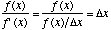
Here, xn is the current known x-value, f(xn) represents the value of the function at xn, and f'(xn) is the derivative (slope) at xn. xn+1 represents the next x-value that you are trying to find. Essentially, f'(x), the derivative represents f(x)/dx (dx = delta-x). Therefore, the term f(x)/f'(x) represents a value of dx.
|


 \end{array}")
}_i = \displaystyle\frac{b_i - \displaystyle\sum_{j=1}^{i-1} a_{ij} x^{(k+1)}_j - \displaystyle\sum_{j=i+1}^{n} a_{ij} x^{(k)}_j }{a_{ii}}")
 derived by extrapolating the
 denotes a Gauss-Seidel iterate and
 ![x^((k))=(D-omegaL)^(-1)[omegaU+(1-omega)D]x^((k-1))+omega(D-omegaL)^(-1)b,](http://mathworld.wolfram.com/images/equations/SuccessiveOverrelaxationMethod/NumberedEquation2.gif)


